
The first section provides in-depth background to spherical harmonics and the spectral transform technique by discussing technical aspects and terminology essential to a clear understanding and informed usage of fields archived by JMA. In spectral models, the spectral space representation of fields is tightly coupled to the corresponding physical latitude-longitude transform grid (a Gaussian grid), and vice versa. The second section discusses the JRA-25 transform grid, which in this case is a regular Gaussian grid. The final section provides a brief description of the regular 1.25° and 2.5° latitude-longitude grids.
Contents
 in spherical
harmonics is written as a double summation
in spherical
harmonics is written as a double summation
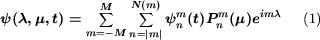
over a truncated wavenumber space where  is the zonal (east-west) wavenumber,
and
is the zonal (east-west) wavenumber,
and  can be regarded as a "total" wavenumber whereby
 gives the number of zeroes between the poles (not including the poles)
of the spherical harmonic function
gives the number of zeroes between the poles (not including the poles)
of the spherical harmonic function  . Hence,
can be interpreted as a type of meridional (north-south) wavenumber.
In the spherical harmonic expansion, the coordinate variables are represented by
. Hence,
can be interpreted as a type of meridional (north-south) wavenumber.
In the spherical harmonic expansion, the coordinate variables are represented by  where
where  is longitude,
 (
( being latitude)
and
being latitude)
and  time. (We have omitted a vertical coordinate for simplicity
of presentation.) In addition, the polynomials defined by
time. (We have omitted a vertical coordinate for simplicity
of presentation.) In addition, the polynomials defined by
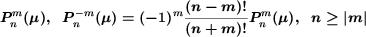
are associated Legendre polynomials of order and degree
, and
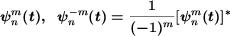
are complex-valued spectral coefficients where  is the
complex conjugate operator. Finally, for simplicity of presentation we set
is the
complex conjugate operator. Finally, for simplicity of presentation we set  ,
resulting in a single constant spectral truncation parameter
,
resulting in a single constant spectral truncation parameter  which
corresponds to what is commonly referred to as triangular truncation. (The usual convention is
to use
which
corresponds to what is commonly referred to as triangular truncation. (The usual convention is
to use  rather than
to designate triangular truncation.) In the
(
rather than
to designate triangular truncation.) In the
( ) wavenumber space
prescribes a triangular region of spherical harmonic modes indicated by the filled circles in the diagram below.
Modes outside of this triangle are set to
) wavenumber space
prescribes a triangular region of spherical harmonic modes indicated by the filled circles in the diagram below.
Modes outside of this triangle are set to  (open circles).
| Spherical Harmonic Wavenumber Space |
|---|
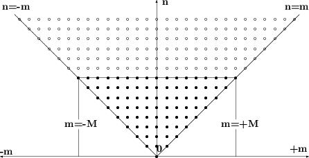 |
Other types of truncation may also be used, such as rhomboidal, but triangular truncation is the most common and is used in ERA-40 (ECMWF, 2002), and for example the NCAR CCM (Kiehl et al., 1998) and CSM (Boville and Gent, 1998). Triangular truncation is frequently referred to as isotropic in the sense that every position and direction on the sphere is treated identically, that is, spectral solutions obtained using triangular truncation are invariant with respect to a coordinate rotation. Washington and Parkinson (1986), and Hack (1992), discuss many aspects of spectral truncation in more detail.
Equation (1) represents the spectral synthesis of a scalar field  from a truncated series of spectral coefficients
  and spherical harmonic functions
. Conversely, in a spectral analysis stage, the spectral coefficients are
obtained by a discretized version of
and spherical harmonic functions
. Conversely, in a spectral analysis stage, the spectral coefficients are
obtained by a discretized version of
 |
 |
 |
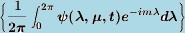
where the inner integral (highlighted in light blue)
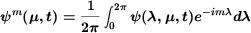
is a forward Fourier transform applied in the zonal (east-west) direction. The forward Fourier transform is computed at each circle of latitude using a discrete fast Fourier transform (FFT). The outer integral
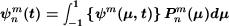
is evaluated in the meridional (north-south) direction using Gaussian quadrature
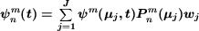
where  denotes Gaussian grid points in the meridional
direction,
denotes Gaussian grid points in the meridional
direction,  the corresponding Gaussian weight at point
, and
the corresponding Gaussian weight at point
, and  the number
of Gaussian grid points in the meridional direction. The
are given by the roots of the Legendre polynomial
the number
of Gaussian grid points in the meridional direction. The
are given by the roots of the Legendre polynomial  and
the by
and
the by
The Gaussian grid points are synonymous with Gaussian
latitudes  , the relation being
  ,
and the number of Gaussian grid points
is synonymous with the number of Gaussian latitudes.
,
and the number of Gaussian grid points
is synonymous with the number of Gaussian latitudes.
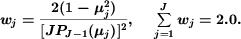
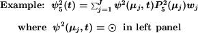
The spectral analysis stage represented by Equation (2) can for illustrative purposes be constructed sequentially from two
arrays as shown in the following diagram. If we choose  equally
spaced longitudes and Gaussian latitudes, then to the columns of the array in the left panel
we assign the FFTs, one for each circle of latitude. The length
of the FFTs is
equally
spaced longitudes and Gaussian latitudes, then to the columns of the array in the left panel
we assign the FFTs, one for each circle of latitude. The length
of the FFTs is  (due to the Nyquist frequency limit, only
half of the possible Fourier modes are retained,
(due to the Nyquist frequency limit, only
half of the possible Fourier modes are retained,
 ,
and the Fourier "mode"
,
and the Fourier "mode"  is the mean value of
  at and time
). In the array in the right panel, we store the spherical harmonic spectral coefficients
at and time
). In the array in the right panel, we store the spherical harmonic spectral coefficients
 obtained by Gaussian quadrature of the Fourier coefficients
 , associated Legendre polynomials
  ,
and Gaussian weights . As an example, we show the how the
,
and Gaussian weights . As an example, we show the how the
 spectral coefficient is computed from the sum of the products of
 (the
(the  in the left
panel),
in the left
panel),  , and .
(In passing we note that
, and .
(In passing we note that  represents the average value of
 at time
  and fixed level.)
| Array of Complex Fourier Coefficients  |
Array of Complex Spherical Harmonic Spectral Coefficients |
|---|---|
 |
 |
 |
|
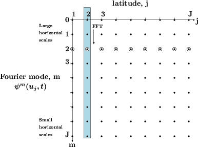
Observe that the dimensions of the spectral coefficient array in the right panel are  , and
that a triangular truncation has been applied. Also, keep in mind that there
are no modes to compute in the
, and
that a triangular truncation has been applied. Also, keep in mind that there
are no modes to compute in the  region, as
  for the associated Legendre polynomials
  . Hence, values of the spectral
coefficient array at () indices outside of the light-gray region need not be computed
and are set to . In general, the triangular truncation
is chosen such that
. Hence, values of the spectral
coefficient array at () indices outside of the light-gray region need not be computed
and are set to . In general, the triangular truncation
is chosen such that  ,
or
,
or 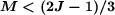 where is the
number of east-west grid points, to avoid aliasing potentially extraneous small spatial scales onto large spatial
scales. (However, this is not to say that modes beyond
where is the
number of east-west grid points, to avoid aliasing potentially extraneous small spatial scales onto large spatial
scales. (However, this is not to say that modes beyond  cannot be
or are not computed — indeed, modes beyond may be retained
depending on the post-processing conventions of the operational, reanalysis, or modeling center, with the
implicit understanding that the appropriate truncation was applied during model integrations.)
cannot be
or are not computed — indeed, modes beyond may be retained
depending on the post-processing conventions of the operational, reanalysis, or modeling center, with the
implicit understanding that the appropriate truncation was applied during model integrations.)
Once spectral coefficients are obtained during a spectral analysis stage, the equivalent physical
representation can be obtained by a spectral synthesis via Equation (1). To follow up on our example,
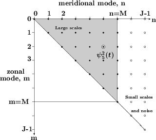
we may choose to focus on only a single mode such that 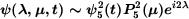 .
The real part of the
.
The real part of the  spherical harmonic function is shown in the following figure. Noting that
  we observe a pattern of alternating negative and positive regions with zonal wavenumber 2 (with nodes at ±45°E and
±135°E) and 3 meridional nodes at 0°N and ±35.3°N. Of course, in a complete
spectral synthesis we are summing over many different spherical harmonic modes (multiplied by the corresponding
spectral coefficient).
we observe a pattern of alternating negative and positive regions with zonal wavenumber 2 (with nodes at ±45°E and
±135°E) and 3 meridional nodes at 0°N and ±35.3°N. Of course, in a complete
spectral synthesis we are summing over many different spherical harmonic modes (multiplied by the corresponding
spectral coefficient).
| Real part of Spherical Harmonic Function |
|---|
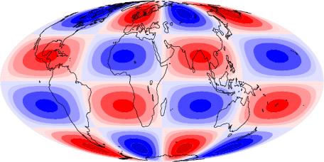 |
 blue represents negative values, red positive values
 |
Equations (1) and (2) (spectral synthesis and spectral analysis) constitute a transformation pair in which a
scalar variable at time
may be represented in physical space, Equation (1), or spectral space, Equation (2).
Both are equivalent representations of and each possess
context-dependent computational advantages and disadvantages. The transformation pair is bound together by
the transform grid, constituting the physical, or grid-point space, defined by the
Gaussian latitudes and equally spaced longitudes.
Throughout the preceding discussion, we have chosen to emphasize the time-dependent nature of the scalar
variable by adhering to notation that retains explicit reference
to time, especially in the spectral coefficients . This allows
us to conclude this section by discussing the broad outline of a typical forecast (integration) cycle in
modern spectral GCMs.
GCMs have as their basis the primitive equations which describe atmospheric dynamics
and thermodynamics employing six equations in six unknowns — three momentum equations relating the east, north, and vertical
components of velocity ( ) to the gradient of pressure
 (Newton's second law of motion in a noninertial reference frame), a mass continuity equation
relating local changes in density
(Newton's second law of motion in a noninertial reference frame), a mass continuity equation
relating local changes in density  to divergence
or convergence of atmospheric mass, a thermodynamic equation
relating temperature
to divergence
or convergence of atmospheric mass, a thermodynamic equation
relating temperature  to the storage and conversion of thermal and other
forms of energy into work (first law of thermodynamics), and an equation of state relating
, ,
and (the ideal gas law).
Through various approximations (e.g. hydrostatic) and combinations, the primitive equations are reduced to a set of model
equations that are of two types, these being prognostic equations of scalar
variables (these predictive variables are hereafter referred to as
prognostic variables), and diagnostic equations of variables that are most
conveniently computed from the prognostic variables. In a typical GCM, the resulting prognostic variables
are vorticity
to the storage and conversion of thermal and other
forms of energy into work (first law of thermodynamics), and an equation of state relating
, ,
and (the ideal gas law).
Through various approximations (e.g. hydrostatic) and combinations, the primitive equations are reduced to a set of model
equations that are of two types, these being prognostic equations of scalar
variables (these predictive variables are hereafter referred to as
prognostic variables), and diagnostic equations of variables that are most
conveniently computed from the prognostic variables. In a typical GCM, the resulting prognostic variables
are vorticity  , divergence
  ,
temperature , and surface pressure
,
temperature , and surface pressure  ,
with specific humidity
,
with specific humidity  added for the inclusion of atmospheric moisture.
The horizontal components of both the prognostic and diagnostic sets of model equations are then subjected to the spectral transform method,
converting these equations to an equivalent representation in spectral space, i.e. in terms of spectral coefficients.
added for the inclusion of atmospheric moisture.
The horizontal components of both the prognostic and diagnostic sets of model equations are then subjected to the spectral transform method,
converting these equations to an equivalent representation in spectral space, i.e. in terms of spectral coefficients.
To examine the outlines of a model forecast cycle let us focus on a single prognostic variable, in this
case vorticity . The prognostic equation for vorticity
contains linear terms  , horizontal derivatives
 , nonlinear terms
  (usually products of individual space- and time-dependent terms), and parameterizations of forcing terms
 . In the spectral method, the forecast cycle begins
in grid-point space at time and involves the point-by-point
multiplication of the individual parts of nonlinear terms, as well as calculation of physical parameterizations
(see lower left panel in diagram below). (Linear operations and horizontal derivatives are to be carried out
exclusively in spectral space.) In the second phase of a forecast cycle (upper left panel), nonlinear terms
and physical parameterizations are transformed to spectral space. The spectral form of nonlinear terms
. In the spectral method, the forecast cycle begins
in grid-point space at time and involves the point-by-point
multiplication of the individual parts of nonlinear terms, as well as calculation of physical parameterizations
(see lower left panel in diagram below). (Linear operations and horizontal derivatives are to be carried out
exclusively in spectral space.) In the second phase of a forecast cycle (upper left panel), nonlinear terms
and physical parameterizations are transformed to spectral space. The spectral form of nonlinear terms
 and physical parameterizations
  ,
as well as the spectral form of linear operations
,
as well as the spectral form of linear operations  and
horizontal derivatives
and
horizontal derivatives  , are then used to compute
the right-hand side of the prognostic equation for vorticity, i.e.
, are then used to compute
the right-hand side of the prognostic equation for vorticity, i.e.  .
In the third phase of the forecast cycle (upper right panel), the spectral coefficients
.
In the third phase of the forecast cycle (upper right panel), the spectral coefficients
 are integrated forward in time one time step
  to time
  . In addition, from the diagnostic set of equations,
the spectral coefficients of the individual parts of nonlinear terms are computed as functions of
(
. In addition, from the diagnostic set of equations,
the spectral coefficients of the individual parts of nonlinear terms are computed as functions of
( ).
).
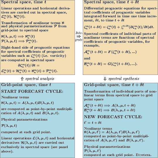
Finally, the forecast cycle is completed by transforming the individual
parts of nonlinear terms from spectral space to grid-point space (lower right panel). In JRA-25,
at time the spectral form of the prognostic variables,
transformed to grid point space, and the grid-point form of parameterized and derived fields are archived
to the physical transform grid — the JRA-25 physical transform grid is the topic of the next section3.
3Our discussion of an integration cycle in a spectral model has purposely omitted reference to data assimilation which combines objective analysis and initialization, key elements in JMA, ECMWF, NCEP, and many other operational and reanalysis programs. (For a brief overview of data assimilation at ECMWF, see pages 462-468 in Holton, 1992).
Contents
Gaussian latitudes and equally spaced longitudes. Choosing
 Gaussian latitudes and
  equally spaced longitudes results in what is referred to (by ECMWF) as a regular
  Gaussian grid4,5.
This is the grid adopted by JMA for JRA-25. The JRA-25 Global Spectral Model (GSM) is summarized below.
Gaussian grid4,5.
This is the grid adopted by JMA for JRA-25. The JRA-25 Global Spectral Model (GSM) is summarized below.
| Specification of the Global Spectral Model (GSM) used in JRA-25 | |
|---|---|
| Equations | Primitive equations with hydrostatic approximation |
| Forecast variables | Vorticity, Divergence, Temperature, Specific Humidity, Cloud Water, Surface Pressure |
| Time integration method | Euler, semi-implicit, leap-frog (3 time levels) |
| Horizontal discretization | Spectral method |
| Horizontal coordinate | Regular Gaussian grid |
| Horizontal resolution | ~1.125°x1.125° (east-west: 125.069 km just north and south of the Equator to 1.874 km near the poles) |
| Number of horizontal grid points | 160x320 (latitude x longitude), latitude 89.142N to 89.142S, longitude 0E to 358.875E |
| Basis functions | Spherical harmonics |
| Truncation wave number | Triangular 106 (T106) |
| Additional details | |
| Assimilation system | Three-dimensional variational (3D-Var) data assimilation (6 hourly) |
| Vertical discretization | Finite difference |
| Vertical coordinate | Hybrid  -pressure coordinate -pressure coordinate |
| Number of vertical levels | 40 (see Hybrid Model Level Coefficients for JRA-25) |
| Pressure of top model level | 0.4 hPa |
| Topography | Defined from GTOPO30 (see USGS 30-second Global Elevation Data, GTOPO30, ds758.0) |
| Land and sea data | United States Geological Survey (USGS) |
| Initialization | Nonlinear normal mode initialization |
| Precipitation parameterization | Prognostic mass-flux Arakawa-Schubert scheme |
| Surface boundary layer | Monin-Obukhov similarity theory |
| Planetary boundary layer | Level 2 Mellor–Yamada turbulence closure model |
| Surface boundary layer | Monin-Obukhov similarity theory |
| Land surface | Simple Biosphere Model (SiB-1) |
| Long wave radiation | Broad-band flux emissivity method (3 hourly) |
| Short wave radiation | Two-stream using -Eddington approximation with eighteen band spectrum (hourly) |
| Gravity wave drag | Long (> 100km, break in stratosphere) and short wave (~10km, trapped and dissipate in troposphere) |
We provide graphical and numerical representations of the regular Gaussian grid
via the following links. The regular Gaussian
grid is used in JRA-25.
, i.e.  ,
convention is used due to the symmetry of the Gaussian latitudes about the Equator.
,
convention is used due to the symmetry of the Gaussian latitudes about the Equator.
5In ERA-40, ECMWF used a reduced
Gaussian grid. See ERA-40 Horizontal Coordinate Conventions
and Numerical Attributes. For Gaussian grids in general, one may intuit that as the pole is approached, the curvilinear distance between meridians of longitude decreases
markedly — e.g. from 125.069 km just north and south of the Equator to 1.874 km near the poles for
regular grids — introducing a distortion in the
area bounded by the four sides of a grid cell. The use of a reduced Gaussian grid, as in ERA-40, alleviates this distortion.
Contents
| latitude spacing | longitude spacing | number latitudes | number of longitudes | first latitude | last latitude | first longitude | last longitude | |
|---|---|---|---|---|---|---|---|---|
| 1.0° | 1.0° | 181 | 360 | 90°N | 90°S | 0°E | 359°E | |
| 1.125° | 1.125° | 161 | 320 | 90°N | 90°S | 0°E | 358.875°E | |
| JRA-25 | 1.25° | 1.25° | 145 | 288 | 90°N | 90°S | 0°E | 358.75°E |
| JRA-25 | 2.5° | 2.5° | 73 | 144 | 90°N | 90°S | 0°E | 357.5°E |
| 5.0° | 5.0° | 37 | 72 | 90°N | 90°S | 0°E | 355.0°E |
We provide graphical and numerical representations of the JRA-25 regular 1.25° and 2.5° latitude-longitude grids via the following links
Contents
Boville, B. A., and P. R. Gent, 1998: The NCAR Climate System Model, version one. J. Climate, 11, 1115-1130.
Bourke, W., 1972: An efficient, one-level primitive-equation spectral model. Mon. Wea. Rev., 100, 683-689.
Eliasen, E., B. Machenhauer, and E. Rasmussen, 1970: On a numerical method for integration of the hydrodynamical equations with a spectral representation of the horizontal fields. Rep. No. 2, Institut for Teoretisk Meteorologi, Københavns Universitet, Copenhagen, Denmark, 35 pp.
ECMWF (European Centre for Medium-Range Weather Forecasts), 2002: The ERA-40 Archive. Reading, ECMWF, 40 pp. (On-line and A4 PostScript versions are available from the ECMWF ERA-40 Project Plan link.)
Hack, J. J., 1992: Climate system simulation: basic numerical and computational concepts. Climate System Modeling, K. E. Trenberth, Ed., Cambridge University Press, 283-318.
Hack, J. J., and R. Jakob, 1992: Description of a global shallow water model based on the spectral transform method. NCAR Tech. Note NCAR/TN-343+STR, 39 pp.
Hack, J. J., B. A. Boville, B. P. Briegleb, J. T. Kiehl, P. J. Rasch, and D. L. Williamson, 1993: Description of the NCAR Community Climate Model (CCM2). NCAR Tech. Note NCAR/TN-382+STR, 108 pp.
Haurwitz, B., 1940: The motion of atmospheric disturbances on the spherical earth. J. Mar. Res., 3, 254-267.
Holton, J. R., 1992: An introduction to Dynamic Meteorology. Second Edition. Academic Press, 511 pp.
Hortal, M., and A. J. Simmons, 1991: Use of reduced Gaussian grids in spectral models. Mon. Wea. Rev., 119, 1057-1074.
JMA (Japanese Meteorological Agency) Japanese 25-year ReAnalysis (JRA-25) and JMA Climate Data Assimilation System (JCDAS)
Kiehl, J. T., J. J. Hack, G. B. Bonan, B. A. Boville, B. P. Briegleb, D. L. Williamson, and P. J. Rasch, 1996: Description of the NCAR Community Climate Model (CCM3). NCAR Tech. Note NCAR/TN-420+STR, 152 pp.
Kiehl, J. T., J. J. Hack, G. B. Bonan, B. A. Boville, D. L. Williamson, and P. J. Rasch, 1998: The National Center for Atmospheric Research Community Climate Model: CCM3. J. Climate, 11, 1131-1149.
Machenhauer, B., 1979: The Spectral Method. Numerical Methods used in Atmospheric Models, Vol. II, GARP Publication Series 17, World Meteorological Organization, Geneva, 121-275.
Onogi, K., J. Tsutsui, H. Koide, M. Sakamoto, S. Kobayashi, H. Hatsushika, T. Matsumoto, N. Yamazaki, H. Kamahori, K. Takahashi, S. Kadokura, K. Wada, K. Kato, R. Oyama, T. Ose, N. Mannoji, and R. Taira, 2007: The JRA-25 Reanalysis. J. Met. Soc. Jap., 85(3), 369-432.
Orszag, S. A., 1970: Transform method for calculation of vector coupled sums: Application to the spectral form of the vorticity equation. J. Atmos. Sci., 27, 890-895.
Sardeshmukh, P. D., and B. J. Hoskins, 1984: Spatial smoothing on the sphere. Mon. Wea. Rev., 112, 2524-2529.
Swarztrauber, P. N., 1993: The vector harmonic transform method for solving partial differential equations in spherical geometry. Mon. Wea. Rev., 121, 3415-3437.
Temperton, C., 1991: On scalar and vector transform methods for global spectral methods. Mon. Wea. Rev., 119, 1303-1307.
Washington, W. M., and C. L. Parkinson, 1986: An Introduction to Three-Dimensional Climate Modeling. University Science Books, 422 pp.
Contents

Contents